![]()
![]()
![]()
![]()
![]()
![]()
![]()
![]()
![]()
![]()
![]()
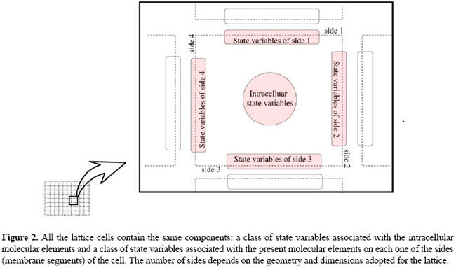
A framework for modeling of juxtacrine signaling systems L.C.S. Rozante1, M.D. Gubitoso2 and S.R. Matioli31Departamento de Ciência da Computação, Universidade Imes, São Caetano do Sul, SP, Brasil 2Departamento de Ciência da Computação, Instituto de Matemática e Estatística, Universidade de São Paulo, São Paulo, SP, Brasil 3Instituto de Biociências, Universidade de São Paulo, São Paulo, SP, Brasil Corresponding author: L.C.S. Rozante E-mail: [email protected] Genet. Mol. Res. 6 (4): 821-845 (2007) ABSTRACT. Juxtacrine signaling is intercellular communication, in which the receptor of the signal (typically a protein) as well as the ligand (also typically a protein, responsible for the activation of the receptor) are anchored in the plasma membranes, so that in this type of signaling the activation of the receptor depends on direct contact between the membranes of the cells involved. Juxtacrine signaling is present in many important cellular events of several organisms, especially in the development process. We propose a generic formal model (a modeling framework) for juxtacrine signaling systems that is a class of discrete dynamic systems. It possesses desirable characteristics in a good modeling framework, such as: a) structural similarity with biological models, b) capacity of operating in different scales of time, and c) capacity of explicitly treating both the events and molecular elements that occur in the membrane, and those that occur in the intracellular environment and that are involved in the juxtacrine signaling process. We have implemented this framework and used it to develop a new three-level discrete model for the neurogenic network and its participation in neuroblast segregation. This paper presents the details of this framework and its current status. Key words: Juxtacrine signaling, Discrete dynamical systems, Neurogenic network INTRODUCTION Signaling systems are an important class of cellular mechanisms that participate in several critical cellular events, such as proliferation, differentiation and apoptosis; these systems are therefore fundamental to developmental programs, influencing the formation of cellular patterns, tissues, organs, and morphogenesis, among others (Wolpert, 1998). Juxtacrine signaling is an intercellular communication based on transmembrane proteins, anchored in the plasma membrane. The two principal types of transmembrane proteins participating in this system are ligands and receptors: a receptor can trigger a series of molecular reactions inside of a cell if it is activated (through a ligand/receptor binding) by a ligand positioned in the membrane of a neighboring cell. As in juxtacrine signaling, both the receptor and the ligand are anchored in the membranes, the activation of the receptor depends on direct contact between the membranes (juxtaposed) of the cells involved. This implies that the ligands act in a more restricted way, only operating on the adjacent cells (immediate neighbors). There are a variety of signaling pathways that are triggered by ligands anchored in the membrane (Fagotto and Gumbiner, 1996). In some cases, juxtacrine signaling seems to be a variant of paracrine signaling, in which ligands anchored in the membrane are virtually the same as those secreted (for instance, growth factors), except for the fact that they contain membrane anchoring domains. In these cases, the anchored ligands are often even precursors of soluble forms that can be easily obtained by proteolytic cleavage (Massagué, 1990). Juxtacrine signaling is vital in several phases of development and maintenance of tissues, for instance, in neurogenesis in Drosophila melanogaster (Castro et al., 2005), in the generation of cellular polarity in ommatidia (Bray, 2000), and in the early development of vertebrates (Lewis, 1998), among others. It actively participates in the processes of cellular patterning. The two main mechanisms that operate in systems of juxtacrine signaling for the formation of patterns are lateral inhibition and lateral induction. We will use the term lateral inhibition to identify interactions of the cell-cell type that cause a cell to choose a certain fate, and, at the same time, to inhibit the neighboring cells from following the same fate. The term lateral induction will be used for the reverse mechanism of lateral inhibition; that is, identify interactions that lead a cell to choose a fate, and, at the same time, to induce neighboring cells to follow the same fate. Good models of systems of juxtacrine signaling must be able to represent these mechanisms and to reproduce spatio-temporal expression patterns observed in many cellular events, especially in the development process. The first, and well-referred, formal model for juxtacrine signaling (Collier et al., 1996) was formulated in terms of the activity of the ligand Delta and its receptor Notch. In this model the mechanism of lateral inhibition was described through a feedback loop through which small differences among neighboring cells are amplified and consolidated. In their study, Collier et al. proposed a set of differential equations to control the rate of production of these proteins. Owen and Sherratt (1998); Owen et al. (2000); Wearing et al. (2000), and Wearing and Sherratt (2001) improved previous models, instead of adopting an arbitrary measure of the activity of the proteins as parameter; they suppose that the variables of the model are the amount of free ligand molecules, the amount of free receptor molecules, and the amount of ligand/receptor complexes formed on the surface of the cell. According to these models, these variables govern (by inhibiting or inducing) the production of new ligands and receptors, consequently promoting lateral inhibition or lateral induction. There are several studies (Owen et al., 1999; Wearing and Sherratt, 2001; Owen, 2002; Webb and Owen, 2004b) that analyze the behavior of these models and the pattern type generated in several geometries of cells (square, hexagonal, etc.). Most models proposed for juxtacrine signaling are essentially continuous. Some are continuous in both space and time (Owen and Sherratt, 1998), others are continuous in time but discrete in space (Monk, 1998; Owen et al., 2000; Wearing et al., 2000). Luthi et al. (1998) proposed a model for juxtacrine signaling that is discrete in both space and time which consists primarily of a cellular automaton with continuous state variables. The most recent model for juxtacrine signaling (Webb and Owen, 2004a) incorporated the treatment of inhomogeneous distribution of receptors in the cell membrane. It is an extension of the model proposed by Owen and Sherratt (1998); Owen et al. (2000); Wearing et al. (2000), and Wearing and Sherratt (2001), adding relative terms to the diffusible transport of proteins between segments of membrane of the same cell as well as modifying the feedback functions so that the localized production of ligands and receptors was considered. We defined a juxtacrine signaling system (JSS) as the set formed by the molecular elements, including their interactions and the molecular mechanisms that participate in the process of juxtacrine signaling. These elements and mechanisms can be intracellular - for instance, signal transduction pathways or gene regulatory networks - or associated with the membranes of the cells in the communication process, for instance, binding events between ligands and receptors positioned in the membrane. The principal existing models for JSS can be divided into three groups: the models of activity, for instance, the model of Collier et al. (1996); the ligand-receptor models, for instance, the model of Owen and Serratt (1998) and Owen et al. (2000), and the segmental models, for example the model of Webb and Owen (2004a). All these groups are based on differential equations, which makes them difficult to analyze if the number of dependent variables grows, since they demand the knowledge of many experimental parameters, which are typically not available. Except for the model type proposed by von Dassow et al. (2000) and von Dassow and Odell (2002), they simplify the participation of the components and intracellular mechanisms involved in the process of juxtacrine signaling, for instance, the participation of certain critical genes and their corresponding regulation mechanisms; that is, these models do not describe in a detailed manner how these intracellular components operate in the signaling process. This is done by encoding the influence of the intracellular components in feedback functions, which makes these models focus on the binding events that occur in the membrane. Models discrete in both time and space, for instance, the model of Luthi et al. (1998), also do not explicitly capture the intracellular molecular interactions that occur in the process of juxtacrine signaling. JSS was designed to allow a natural and intuitive mapping of the real, biological system into an abstract mathematical model. This makes the translation back and forth easier and less error prone. Therefore, a model must have the capacity to represent several elements and their time evolution present in JSS and must be rich and sufficiently comprehensive to capture several types of molecular events (intra- and extracellular) that occur in the process of juxtacrine signaling, for instance, conformational modifications in membrane proteins, protein-protein interactions that can occur in the membrane or inside the cell, transcription, translation, dependence between genes, and post-translational modifications. A model should also have the capacity of modular representation of the signaling systems, since the complexity of the signaling and regulation networks suggests that its analysis demands that the modeling methods be capable of treating parts of the network as modules and several signaling networks present groups of elements and mechanisms that show operation and modular organization (Bruggeman et al., 2002). It is also important that the system must be capable of working over several orders of magnitude in spatio-temporal scales, because signaling cellular networks operate with events whose responses vary from tenths or hundredths of a second (for instance, protein modifications) to several minutes (transcriptional and translational regulation, for example) (Papin et al., 2005) and finally allowing for the integration of experimental data of different types and sources. Although continuous time models allow a more detailed description of the variation rates involved (for instance of mRNA concentration and proteins), as already mentioned, they demand the knowledge of experimental data not always available (for instance values of kinetic constants). In addition, the discrete modeling of signaling systems (Allen et al., 2006) and of regulation (Thomas, 1973; Albert and Othmer, 2003) is already a relatively well-established activity. In the following sections, we describe a framework of discrete modeling of JSS that, at the same time, contemplates some of the characteristics mentioned above and can be used in several situations and applications, in the context of the juxtacrine signaling process. DESCRIPTION OF FRAMEWORK (METAMODEL J ) We propose a general formal model for JSS called metamodel J, as a class of dynamical systems with discrete time and space and state variables which may be discrete or continuous. An overview of J In J, a tissue structure is represented by a regular lattice, whose elements, denominated cells, have a 1:1 correspondence with live cells, as shown in Figure 1. A lattice cell is an autonomous entity whose state is defined by the state of its intracellular components and membrane components. 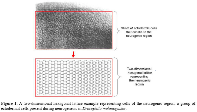 The intracellular components of a lattice cell are a class of state variables that represent the states of the intracellular molecular elements of the living cell. The components of the lattice cell membrane are another class of state variables, which are divided into subclasses, and each subclass is associated with a side (membrane segment) of the cell. The membrane components represent the states of the molecular elements that are present in the segments of plasma membrane of the living cell, as shown in Figure 2.
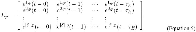
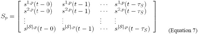
All the lattice cells contain the same components (intracellular and membrane) and their states, for each discrete time step, are determined by the application of the same transition rules valid for every lattice cell. The transition rules can be classified as intracellular (those that update the intracellular components) and membrane (those that update the membrane components). The intracellular components along with their transition rules represent the signaling nets and show intracellular regulation in the living cell. The membrane components along with their transition rules represent the signaling mechanisms that operate in the plasma membrane of the living cell. A more detailed view of J An M model in J corresponds to a dynamical system whose general form is M = (R,V,I,T ), where R is a regular lattice, V is a finite set of variables associated with each element of R, I is a set of initial conditions associated with V, and T is a set of transition rules. In the following sections, the properties and restrictions that define these components are better described. Lattice characterization A regular lattice R is a finite periodic network of elements, denominated cells, in a (finite) space of dimension d that is completely filled out by the cells. The elements that characterize a lattice are: a) its dimensions (1D, 2D or 3D); b) its size, i.e., its number of cells; c) its topology, and d) the boundary conditions, namely the number of neighbors of the cells that are located at the extremities (borders) of the lattice. The boundary conditions are used to determine, for instance, whether a cell located on the left border of a lattice has neighbors to its left or not. In J, these conditions are restricted to two cases: periodic or linear. The periodic boundary consists of identifying the lattice on its lateral boundary so that the cells of the opposite borders of the lattice are neighboring each other, so that it is close or simulates the situation where it is laterally completed. That makes every cell have the same amount of neighbors. The linear boundary (or of fixed values) has fixed values for the present cells in the boundary of the lattice. The value to be attributed should carry the information so that the cell does not possess the same amount of neighbors as those positioned in the interior of the lattice. Characterization of the cells and of V set Given a lattice R, a cell in R is identified by its relative position p, represented by a point in the coordinated axes: p = (x) ∈ N (for one-dimensional lattice), p = (x) ∈ N² (for two-dimensional lattice) or p = (x) ∈ N³ (for three-dimensional lattice). In addition to its identifier, each cell p in R contains a set of variables V = {E,G,S,B,A}. E, G and S are finite sets of variables representing, respectively, the intracellular signaling and gene regulatory network input (intracellular network input for short), the intracellular metabolites and gene state in the intracellular signaling and gene regulatory network (intracellular network state) and intracellular signaling and gene regulatory network output (intracellular network output). An element ek ∈ E is called input and ek(t) ∈ E is called input value of ek at time t, t ∈ T, where T ⊂ N denotes the domain of the discrete time and E ⊂ R is the set of the possible values that an input can assume. We represented the several values of input ek(t) by a two-dimensional vector E. Similarly, an element gk ∈ G is called state and gk(t) ∈ G is called state of at gk time t, t ∈ T, where G ⊂ R is the set of the possible states that a gene or intracellular metabolite can assume. Accordingly, the states gk(t) are represented by a two-dimensional vector G. In the same way, sk∈ S is called output and sk(t) ∈ S is called output value of sk at time t, t ∈ T, where S ⊂ R denotes the set of the possible values that an output can assume. We represented the various output values sk(t) by a two-dimensional vector S. These vectors are described in the Appendix. Associated with each cell in R, there is a finite set F ⊂ N+ of segments representing the sides of the cell. The number |F | of sides of a cell depends on the geometry and the dimensions of the lattice. To each side f ∈ F of each lattice cell, two finite sets of variables are associated: Bf , named state of transmembrane signaling, and Af , representing the state of environmental signaling. Following the same notation as above, Definition of the initial conditions The third component of an instance of J corresponds to the set I of initial conditions, from which the evolution of the system occurs. The set I is defined as being the value that each variable, in each cell of R and on each side, assumes in the initial instant. State transitions The state transition rules T, valid for every cell in M, can be divided into the following classes: Class Ψ The updating of the state vector G, for every cell p∈R, at each time step, is made by a finite vector of functions Y = [ψ 1, ψ2 , … , ψ |G| ,] where Ψk denotes how the gene and/or intracellular metabolite gk, 1≤k≤|G|, is updated in time. In other words, it describes how the variable of state gk (for every p∈R) evolves in discrete time steps. The functions Ψk:Gτ+1 × Eτ+1→ G are called functions of transition of the intracellular network and are of the form
where 1≤u,v≤|G|, 1≤q,r≤|E|, gk(t)∈G, ek(t)∈E and 0≤x,y≤τ, where τ corresponds to the earliest time used by Ψk.
Class Φ Similarly, the updating of the vector of outputs S is made by a finite vector Φ = [Φ1,Φ2 , … ,Φ|S| ], where Φk denotes how the output k, 1≤k≤|S |, of the intracellular network is updated in time, in other words, it describes how the variable of output sk (for every cell p∈R) evolves in discrete time steps. The functions Φk:Gτ+1×Eτ+1→S are called functions of output of the intracellular network and are of the form
where 1≤u,v≤|G|, 1≤q,r≤|E|, Class Θ The updating of the vectors of states Bp,f, 1≤f≤|F | and p∈R , is made by the vector Θ = [θ1,1 , … , θ1,F , … , θ2,1 , … , θ2,F , … , [θ|Bf |,1 , … , θ|Bf |,F], where θj,f denotes how the membrane signaler j, 1≤j≤|Bf |, of side f, is updated in time; that is, it describes how the variable of state The functions
where 1≤k,l≤|S |, 1 ≤ q,r ≤ |Af |, 1≤ m,n ≤ |Bf |, z,w∈V(p) = {v : v is neighboring p in R } (that is, z and w are neighboring cells of cell p), 1≤u,v≤|F|, and 0≤x,y≤τ.
The restrictions on the influence relationships, defined by the classes Ψ, Φ and Θ, are summarized in the following way:
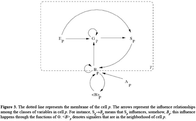
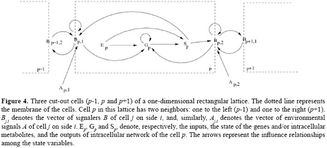
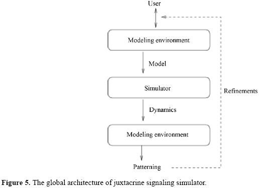
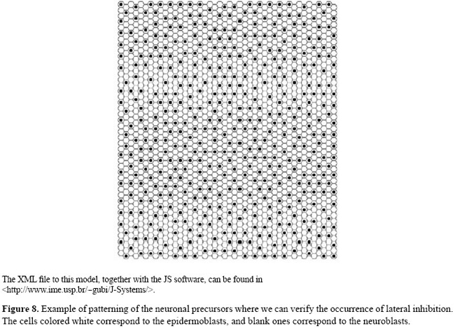
In Figure 3, we present a general schematic representation of these restrictions on the influence relationships among the classes of variables in J, and in Figure 4, we illustrate this representation for the case of the one-dimensional rectangular lattice. Ep represents internal events - a signal of an alternative signaling pathway or the constitutive expression of genes, for instance - and Ap,f represents external events - an environmental signal, for instance, the temperature variation. They represent independent signals and are not explicitly modeled but may alter the state of the variables. Stochastic models in J In J, it is possible to define both deterministic and stochastic models. We denominate an instance of J as being deterministic if only one transition function is associated with each variable of the model. If the model is stochastic, we define a list of functions per variable and we associate a probability with each of the functions. This implies that in the definition of a stochastic model, it is necessary to define a finite set of functions F and a distribution of probabilities PF in F. DEFINITION OF MODELS AND IMPLEMENTARION To describe an instance of J means to define: a lattice, i.e., its size (number of cells), its dimensions (1D, 2D or 3D), its boundary conditions (linear or periodic), and the geometry of its cells; the domain of each one of the sets of state variables; the name and representation (vectors E, G, S, Af and Bf ) of state variables; the initial conditions I, and the type of model (deterministic or stochastic). If the model is deterministic, define the transition functions T; i.e., to define exactly how each one of the functions in Ψ, Φ and Θ is, so that each variable is updated by just one transition function. If the model goes stochastic, the definition of T demands the definition of a finite set of functions F and a distribution of probabilities in F, as described in the previous Section, for each one of the variables of the model. For defining, simulating, analyzing, and refining models in J, we implemented a software called juxtacrine signaling simulator (JS), composed of three modules (see Figure 5): a) a modeling setting; the main components of this module are an interface for edition and visualization of models and a system for verification of their consistency, and b) a simulator of models in J and c) an interface for visualization and analysis of simulations and results, containing several components, such as a viewer of cellular patterns and reports and descriptive graph generators for the state behavior and evolution. Models are edited using modeling setting and are recorded in XML (eXtensible Markup Language; Bray et al., 2000) files. The simulator reads the model in the XML format as input, runs the simulation and provides a set of tables describing the dynamic of the state variables of the model as output. These tables can be used by the interface for visualization and analysis. The code in alpha version of the JS software and a brief manual for installation can be found at <http://www.ime.usp.br/~gubi/J-Systems/>. SBML (Systems Biology Markup Language; SBML, 2007) is a language for the description of models of biological systems based in XML and Unified Modeling Language (Group, 2002) that has been very well known in the last years, being supported by almost 100 different softwares. In this way, it is an important standard for model interchange among packages and tools of simulation/analysis.
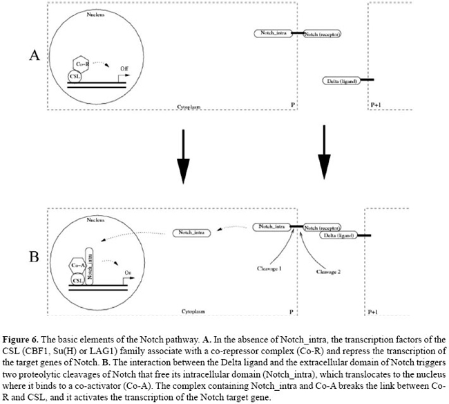
SBML has been developed in levels, where each new level extends, in compatible manner, the features of the language in the previous level. The final version of SBML level 1 (Hucka et al., 2001) presents the basic resources and fundamentals for representation of non-spatial models of biochemical networks. The final version of SBML level 2 (Finney and Hucka, 2003) has been already defined and incorporates facilities for representing some features in the models in J, as example the capability of definition of "delay functions" and "discrete events". However, class J contains models that cannot be codified in SBML level 2, since it does not support models spatially dependent in which each biological entity is univocally identified and individually defined. Several proposals for the extension of SBML level 2 have been offered (see in SBML, 2007) and will likely be incorporated in SBML level 3. The main features that the community plans to incorporate in SBML level 3 that are important to the process of model codification from J to SBML format are: a) arrays of species, compartments and reactions, b) mechanism for describing the connections between items in an array and c) facilities for describing the geometry of compartments in 2-D and 3-D spaces. Some models featured in J could be already mapped to entities described in proposals of extensions of SBML level 2, for example: a) a state variable in J could be mapped to a species in SBML; b) a transition function in J could be mapped to a reaction in SBML, c) a cell in J could be mapped to a compartment in SBML, and d) a lattice in J could be mapped to an array of compartment in SBML. Our intention in the future is to build a parser (to be integrated to the JS software) that would be able to translate models in the J format to the SBML format. The JS software operates with XML pattern that helps this task; however, we believe that it is not convenient to build it until the final version of SBML level 3 is defined. Applications Due to its generality, the metamodel J can have several applications in different contexts, for instance: a) in the modeling and analysis of formation of patterns in juxtacrine signaling; b) in the study of methods of identification of units of signaling and metabolic pathways induced by environmental signals; c) in the simulation of cellular juxtacrine signaling and regulation networks, and d) in the reconstruction and in the structural and dynamic analysis of networks of juxtacrine signaling. In the following sections we showed the application of J in the modeling of the elements and basic interactions (extracellular and intracellular) that participate in neuroblast segregation in D. melanogaster. NOTCH PATHWAY The Notch pathway is a vital signaling pathway, present in several events in the development of several organisms, e.g., in neurogenesis in Drosophila (Castro et al., 2005), in the early development of vertebrates (Lewis, 1996, 1998; Whitfield et al., 1997), and in the establishment of boundaries between veins and interveins in the Drosophila wing (Huppert et al., 1997). Signaling of the cell-cell type, mediated through the Notch pathway, is a mechanism that operates in several situations where there are definitions of cell fate. Notch is particularly effective for establishing the binary cell fate between two or more adjacent cells or nearby cells, which occurs basically in three general settings: lateral inhibition (Parks et al., 1997); communication of juxtaposed rows of cells where each row adopts a distinct fate (Bessho and Kageyama, 2003), and binary choice of fate among sister cells in asymmetric cell divisions (Kim et al., 1996). We will briefly describe the main molecular characteristics (schematized in Figure 6) of the Notch pathway. Its essential elements are a ligand of the Delta type, a receptor of the Notch type and a transcription factor of the CSL (CBF1, Su(H) or LAG1) family. The basic mechanisms of this pathway are highly conserved and they have been already identified and studied in several species, for instance, in C. elegans, D. melanogaster and in some mammals (Lai, 2004). The Delta and Notch are transmembrane proteins that contain an extracellular domain constituted of arrays of epidermal growth factor repeats. Specific epidermal growth factor repeats mediate the interaction between the ligand and the receptor. The activation of Notch for its corresponding ligand triggers two proteolytic cleavages of Notch: one in its extracellular domain and another in its intracellular domain. The intracellular domain (Notch_intra) translocates from the membrane to the nucleus where it activates the transcription factor (CSL). In the absence of Notch_intra, CSL binds to a co-repressor forming a complex that inhibits the expression of the target genes of Notch. In the presence of Notch_intra, CSL binds to a co-activator forming a complex that induces the activation of the target genes of Notch. Figure 6 displays a schematic representation of this mechanism. Delta-Notch and neurogenesis in Drosophila melanogaster One of the best known examples in which the Notch pathway operates, is in the formation of the nervous system in Drosophila, more specifically in the processes of neuroblast segregation and determination of sensory organ precursor cells (that give rise to the sensory bristles of the epidermis). Soon after gastrulation, the cells of the neurogenic region (an area of approximately 1900 ectodermic cells formed by two longitudinal strips of cells along the anteroposterior axis of the embryo, in a position slightly dorsal in relation to the ventral mesoderm) assume a bipotential character: they can become neuroblasts - precursors of neural cells - or epidermoblasts, which are the precursors to the epidermis. The distribution of the neuroblasts and epidermoblasts in the neurogenic region, after each cell has assumed its fate, depends on elements of intracellular regulation and cell-cell interaction.
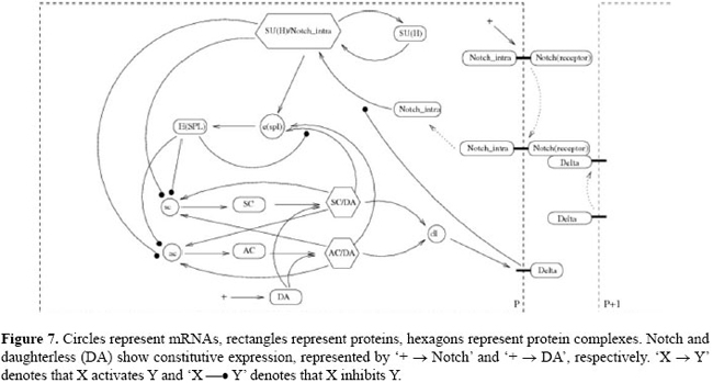
The proneural genes (mainly of the achaete-scute complex) assign to the ectodermic cells the potential for becoming neural precursors. In the neurogenic region, cells expressing these genes become clusters of cells (called proneural clusters). Not all the cells of one neural cluster become neuroblasts, and the process that leads to its specification involves lateral inhibition. Therefore, after the formation of the clusters, all the cells in the clusters have the potential for becoming a neuroblast, until one of them (the future neuroblast) begins to express - through a random event - genes of the achaete-scute complex in higher levels than the others. This implies that this cell produces a signal, transmitted through juxtacrine interactions between Delta and Notch, which inhibits its neighbors from becoming neuroblasts, by making it a neural precursor and the remaining cells of the cluster become epidermal epithelial cells. Regarding the molecular interactions that modulate the expression of Delta and Notch, many studies (Bailey and Posakony, 1995; Paroush et al., 1997; Meir et al., 2002; Lai, 2004) suggest that several genes and proteins can participate in the transmission and adjustment of the Notch signal. However, we will limit the description to the best established components and connections, which we will call the "canonical neurogenic network", or simply "canonical network". The architecture of this regulation network, its principal components and its interactions are schematized in Figure 7. Its main characteristics (Bailey and Posakony, 1995; Paroush et al., 1997; Meir et al., 2002; Lai, 2004) can be summarized as follows.
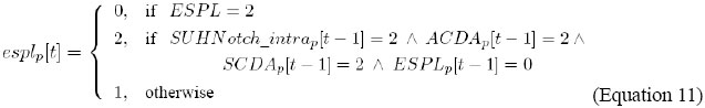
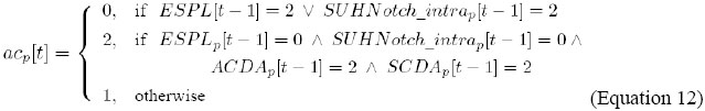
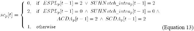
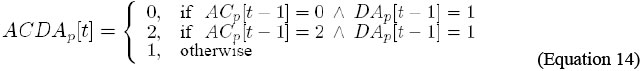
Delta is the ligand for the Notch receptor and when Delta activates Notch the intracellular domain of Notch (Notch_intra) links to the suppressor of hairless (SU(H)) transcription factor, which is from the CSL family, to form the dimer SU(H)/Notch_intra. Then, SU(H)/Notch_intra activates the transcription of the genes of the enhancer of split (e(spl)) complex, which codify for the transcriptional repressor E(SPL), which in its turn represses the transcription of the proneural genes achaete (ac) and scute (sc), the primary determinant of the neural fate: cells with high concentrations of the products AC and SC become neuroblasts; AC and SC are transcription factors that contain a conserved motif of the basic helix-loop-helix type. They use the basic helix-loop-helix domain for dimerizing with other factors, becoming active as dimers. AC and SC each link to the daughterless (DA) co-factor and, in the heterodimer state (AC/DA and SC/DA), they activate the transcription of each other and of the other (see Figure 7). AC/DA and SC/DA also activate the transcription of the dl gene (which codifies for the Delta ligand) and of the e(spl) gene, whose product (E(SPL)), as previously mentioned, represses the ac and sc transcription. Thus, a loop is formed: a random event activates ac and/or sc in a cell of the proneural cluster. They activate dl, whose product (Delta) activates Notch in the neighboring cells, in which, through the complex SU(H)/N, e(spl) is activated, which consequently, represses ac and sc. Besides this, it must be taken into account that Delta represses the activity of Notch in the cell itself, e(spl) also promotes autorepression, and the genes for Notch and DA show constitutive expression. A three-level model in J for delta-Notch system Based on the architecture of the suggested canonical network, we built a new deterministic J model for neuronal precursor patterning. It is formulated in terms of the levels of activity of the genes, of the proteins and of the complexes involved, and its description is as follows. We mapped the cells of the neurogenic region in a two-dimensional lattice R with periodic boundary conditions and containing 1936 hexagonal cells. In relation to the domains, we let E = {0,1,2}, G = {0,1,2}, S = {0,1,2}, and Bf = {0,1,2}. Regarding the variables, to maintain adherence to the notation of Figure 7, we took the following steps: a) set E = {e1,e2} which we used to represent the constitutive expression of Notch and DA, respectively; b) set G = {Notch_intra, SUHNotch_intra, espl, ESPL, ac, sc, AC, SC, ACDA, SCDA, dl, DA, SUH}, where each variable in G denotes the level of the corresponding component intracellular homonymous activity, for instance, Notch_intra denoting the level of activity of Notch_intra (intracellular domain); c) does not include environmental signals in the model; d) set S={s1}, in which we attributed the level of dl activity, and e) with no discrimination on the sides of the cells, i.e., we assumed that each cell has only one side (F = {1}), so that in each cell we have only one set of signalers B1 = {Delta, Notch, Notch_Delta}. We detailed these definitions in the Appendix. To represent the initial state, we assigned to every cell, at t = 0, the value "1" for all the state variables. The transition rules are functions in the combination of states (in the previous instant) of the affectors that are incident on components. For instance,
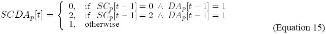
It indicates that the state of dl, in cell p, is updated by a combination of states of SC/DA and AC/DA, in cell p, in the previous instant (t-1). The states 0/1/2 denote, respectively, low/medium/high level of activity; for instance, ACDAp[t]=2 means that AC/DA has a high level of activity in cell p and in the current instant. In the Appendix, we detailed the transition rules for each one of the components of the model. We performed some preliminary experiments simulating the process of neuronal precursor segregation. For this, we assumed that there are two interesting states in the model: the initial state, corresponding to the situation in which all the cells are bipotents, and the final, corresponding to the situation in which the neuroblasts are segregated. Once we simulated the model, we observed that the system remained in the steady state regarding the initial conditions (bipotent cells). In the sense used by Wuensche (1998), this state and its attraction basin correspond to a cell type. We then introduced (by independent signals) several flotations in the state of some model component, starting from the initial state. We used these flotations in order to reproduce in silico the best results in wet experiments well described in literature. At first, we chose a random cell from the neurogenic region and we increased the expression levels of ac and sc. As expected this cell becomes a pro-neural precursor (defined by the Delta state) and in time it inhibits its neighbors from changing in the same way. In these conditions, the system enters a stationary state, which suggests that this state and its attraction basin correspond to another cell type and that the trajectory followed by the model represents the related differentiation pathway. Afterwards, we performed simulations varying the levels of ac and sc expression in random cells and at random timesteps. In these cases, we observed that:
DISCUSSION AND CONCLUSION The organization adopted for the metamodel in J was designed to possess a structure similar to the one of the models commonly used by the biology community for JSS, since we consider this a desirable characteristic. We expect that the structure of the lattice (where each cell is an autonomous entity with the same components) representing the tissues, the grouping of the state variables as intracellular and of the membrane and the imposed restrictions in the transition rules (distinguishing the representation of the events that occur in the membrane from those that occur in the intracellular medium), could offer the similarity that we seek. The formal models for JSS developed so far focus on the binding events between ligands and receptors that occur in membranes of communicating cells. J is capable of representing the participation of the intracellular components, which extends the representation power of the current JSS models, allowing the most detailed representation of the several structures (membrane and intracellular ones) and showing interactions in the transduction pathways, especially those related to gene regulation involved in the formation of patterns in juxtacrine signaling. The capacity to operate with different scales of time is guaranteed in J through the construction of delay cycles modeled in the system memories. For that, it is necessary to define for the specific model in study its unit of time, that corresponds to a discrete time step. This unit can be defined as being, for instance, the interval of time of the fastest considered molecular event. The "amount of time" of the other considered events will always be proportional (larger than or equal to) the established unit. Good models of juxtacrine signaling should be capable of treating the inhomogeneous distribution of ligands and receptors in the membranes, because it influences polarization events, for instance in dorsoventral polarization in the eyes of Drosophila (Bray, 2000). In this sense, the division of the membrane in segments (sides) adopted in J is important to allow the representation of the located accumulation of proteins, which can occur by local protein synthesis, active transport from intracellular stores and selective degradation (Strutt, 2002). The modular representation of JSS in J can be obtained through the application of methods of modular response analysis (Bruggeman et al., 2002). It enables it to stand up to different models, with different resolutions, for the same signaling system. J can emulate other formal models of juxtacrine signaling, as long as these are originally conceived with the discrete time and space or it can be converted into a discrete approach. We know that numeric methods of resolution of differential equations correspond to conversions of this type; in addition, many systems of differential equations can be approximated by a system of equations of differences. Thus, we conclude that J can be applied in the emulation of a wide range of models, which reinforces its generality. We illustrated the use of J in the modeling of the Delta-Notch system and its participation in the patterning of neuronal precursors. In the simulations, we obtained results compatible with the expected patterns: occurrence of lateral inhibition with 20-30% of the cells having adopted primary fate (neuroblasts) and 70-80% of the cells having adopted secondary fate (epidermoblasts). However, refinements in the model are still necessary, as well as new improved simulations and analysis in order to identify structural and functional properties in the model proposed for the Delta-Notch system. Natural deficiencies of J are those intrinsic to the discrete modeling. In addition, due to its abundant details, the complexity of computational time and space involved can represent a drawback of J, depending on the model type that is created. However, it is interesting to observe that juxtacrine signaling is typical in the initial phases of embryonic development, where the amount of cells is relatively small, where the signaling pathway is typically complex. Although we did not have problems with the simulations that we performed, it is reasonable to suppose that, in situations where the amount of cells is immense, the computational demand can grow swiftly. This suggests that extensions of this study can be related to more efficient computational solutions. For instance, the structure of the model provides a natural ease in performing its paralleling, which could be explored. Other possible extensions for this study include: a) exploring dynamical properties of J models, such as the development of an algorithm for automatic generation of attraction basins for small Boolean models; b) application of J for a more detailed analysis of the Delta-Notch system, which could incorporate multi-level variables and environmental signals, and c) application of J to model and to analyze other biological events, for instance the planar polarity generation in ommatidia (Bray, 2000). Besides, in the near future we intend to build a translator for a model in J to SBML level 3, as soon the specification becomes available. References Albert R and Othmer HG (2003). The topology of the regulatory interactions predicts the expression pattern of the segment polarity genes in Drosophila melanogaster. J. Theor. Biol. 223: 1-18. Allen EE, Fetrow JS, Daniel LW, Thomas SJ, et al. (2006). Algebraic dependency models of protein signal transduction networks from time-series data. J. Theor. Biol. 238: 317-330. Bailey AM and Posakony JW (1995). Suppressor of hairless directly activates transcription of enhancer of split complex genes in response to notch receptor activity. Genes Dev. 9: 2609-2622. Bessho Y and Kageyama R (2003). Oscillations, clocks and segmentation. Curr. Opin. Genet. Dev. 13: 379-384. Bray S (2000). Planar polarity: out of joint? Curr. Biol. 10: R155-R158. Bray T, Paoli J, Sperberg-McQueen CM and Maler E (2000). Extensible markup language (XML) 1.0 (second edition), W3C recommendation 6-October-2000. http://www.w3.org/TR/1998/ REC-xml-19980210. Accessed January 2007. Bruggeman FJ, Westerhoff HV, Hoek JB and Kholodenko BN (2002). Modular response analysis of cellular regulatory networks. J. Theor. Biol. 218: 507-520. Castro B, Barolo S, Bailey AM and Posakony JW (2005). Lateral inhibition in proneural clusters: cis-regulatory logic and default repression by suppressor of hairless. Development 132: 3333-3344. Collier JR, Monk NA, Maini PK and Lewis JH (1996). Pattern formation by lateral inhibition with feedback: a mathematical model of delta-notch intercellular signalling. J. Theor. Biol. 183: 429-446. Fagotto F and Gumbiner BM (1996). Cell contact-dependent signaling. Dev. Biol. 180: 445-454. Finney A and Hucka M (2003). Systems biology markup language: level 2 and beyond. Biochem. Soc. Trans. 31: 1472-1473. Group OM (2002). Unified Modeling Language. http://www.omg.org/uml. Accessed January 2007. Hucka M, Finney A, Sauro HM and Bolouri H (2001). Systems biology markup language (SBML) level 1: structures and facilities for basic model definitions. http://www.sbml.org/. Accessed January 2007. Huppert SS, Jacobsen TL and Muskavitch MA (1997). Feedback regulation is central to Delta-Notch signalling required for Drosophila wing vein morphogenesis. Development 124: 3283-3291. Kim J, Sebring A, Esch JJ, Kraus ME, et al. (1996). Integration of positional signals and regulation of wing formation and identity by Drosophila vestigial gene. Nature 382: 133-138. Lai EC (2004). Notch signaling: control of cell communication and cell fate. Development 131: 965-973. Lewis J (1996). Neurogenic genes and vertebrate neurogenesis. Curr. Opin. Neurobiol. 6: 3-10. Lewis J (1998). Notch signalling and the control of cell fate choices in vertebrates. Semin. Cell Dev. Biol. 9: 583-589. Luthi PO, Chopard B, Preiss P and Ramsden JJ (1998). A cellular automaton model for neurogenesis in Drosophila. Physica D 118: 151-160. Massagué J (1990). Transforming growth factor-α: a model for membrane-anchored growth factors. J. Biol. Chem. 256: 21393-21396. Meir E, von Dassow G, Munro E and Odell GM (2002). Robustness, flexibility, and the role of lateral inhibition in the neurogenic network. Curr. Biol. 12: 778-786. Monk NAM (1998). Restricted-range gradients and travelling fronts in a model of juxtacrine cell relay. Bull. Math. Biol. 60: 901-918. Owen MR (2002). Waves and propagation failure in discrete space models with nonlinear coupling and feedback. Physica D 173: 59-76. Owen MR and Sherratt JA (1998). Mathematical modelling of juxtacrine cell signalling. Math. Biosci. 152: 125-150. Owen MR, Sherratt JA and Myers SR (1999). How far can a juxtacrine signal travel? Proc. R. Soc. Lond. B 266: 579-585. Owen MR, Sherratt JA and Wearing HJ (2000). Lateral induction by juxtacrine signaling is a new mechanism for pattern formation. Dev. Biol. 217: 54-61. Papin JA, Hunter T, Palsson BO and Subramaniam S (2005). Reconstruction of cellular signalling networks and analysis of their properties. Nature 6: 99-111. Parks AL, Huppert SS and Muskavitch MA (1997). The dynamics of neurogenic signalling underlying bristle development in Drosophila melanogaster. Mech. Dev. 63: 61-74. Paroush Z, Wainwright SM and Ish-Horowicz D (1997). Torso signalling regulates terminal patterning in Drosophila by antagonising groucho-mediated repression. Dev. 124: 3827-3834. Systems Biology Markup Language (SBML) (2007). http://www.sbml.org/. Accessed January 2007. Strutt DI (2002). The asymmetric subcellular localisation of components of the planar polarity pathway. Semin. Cell Dev. Biol. 13: 225-231. Thomas R (1973). Boolean formalization of genetic control circuits. J. Theor. Biol. 42: 563-585. von Dassow G and Odell GM (2002). Design and constraints of the Drosophila segment polarity module: robust spatial patterning emerges from intertwined cell state switches. J. Exp. Zool. 294: 179-215. von Dassow G, Meir E, Munro EM and Odell GM (2000). The segment polarity network is a robust developmental module. Nature 406: 188-192. Wearing HJ and Sherratt JA (2001). Nonlinear analysis of juxtacrine patterns. SIAM J. Appl. Math. 62: 283-309. Wearing HJ, Owen MR and Sherratt JA (2000). Mathematical modelling of juxtacrine patterning. Bull. Math. Biol. 62: 293-320. Webb SD and Owen MR (2004a). Intra-membrane ligand diffusion and cell shape modulate juxtacrine patterning. J. Theor. Biol. 230: 99-117. Webb SD and Owen MR (2004b). Oscillations and patterns in spatially discrete models for developmental intercellular signalling. J. Math. Biol. 48: 444-476. Whitfield T, Haddon C and Lewis J (1997). Intercellular signals and cell-fate choices in the developing inner ear: origins of global and of fine-grained pattern. Semin. Cell Dev. Biol. 8: 239-247. Wolpert L (1998). Principles of development. Current Biology Ltd. and Oxford University Press, Oxford. Wuensche A (1998). Discrete dynamical networks and their attractor basins, in Complex Systems’ 98. University of New South Wales, Sydney. APPENDIX Representation of the variables Representation of E We represented the several values of ek(t) input by a two-dimensional vector E of which we will denominate intracellular network input vector. We denoted:
This way, the vector E in the cell p is defined as follows:
Thus, Ep[k][t-x] represents Representation of G We represented the states gk(t) by a two-dimensional vector G of state variables, which will be called intracellular network state vector which denotes the history (state in current and previous steps of time) of the genes and/or metabolite considered in the model. We denoted:
This way, vector G in cell p is defined as follows:
Thus, G p[k][t-x] represents Representation of S We represented the several output values sk(t) by a two-dimensional vector S which we will denominate intracellular network output vector. We denoted:
This way, vector S in cell p is defined as follows:
Thus, Sp[k][t-x] represents Representation of Bf The states of the signalers, in a side f, are represented by a two-dimensional vector Bfof state variables, denominated vector of signaling of side f. We denoted:
This way, the vector Bp,f, that represents the amount and/or concentration and/or activity of the proteins and/or products of cell membrane p on side f, is defined as follows:
Thus, Bp,f [k][t-x] represents bk,p,f(t-x), that is, the signaler state bk, 1≤k≤|Bf |, in cell p, in the side f, in the instant t-x, 0≤x≤τBf, where τBf denotes the memory (the oldest considered instant) of the system for the variables in Bf . Evidently, the number of vectors Bf that each cell contains is the same as the number of cell sides, that, as we have seen, it depends on the geometry and dimensions of the lattice. For instance, if we assume cubic geometry for the cells of the lattice, we will have up to 6 vectors: Bf , 1≤f≤6. Representation of Af The states of the environmental signals, on a side f, are represented by a two-dimensional vector Af of variables, denominated vector of environmental signaling of the side f. We denoted:
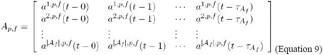
This way, the vector Ap,f is defined as follows:
Thus, Ap,f [k][t-x] represents ak,p,f(t-x), that is, the value of environmental signal ak, 1≤k≤|Af |, in cell p, on side f, at instant t-x, 0≤x≤τAf, where τAf denotes the memory (the oldest considered instant) of the system for the variables in Af . As in the previous case, the number of vectors Af that each cell contains is dependent on the geometry and dimensions of the lattice. Figure 4 provides some insight into the "positioning" of these vectors in the lattice. Details of the definition of the variables and transition rules In order to update the intracellular network input
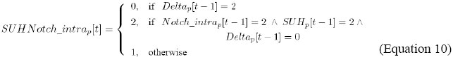
In order to update the intracellular network state (genes and/or intracellular metabolites) G = {Notch_intra, SUHNotch_intra, espl, ESPL, ac, sc, AC, SC, ACDA, SCDA, dl, DA, SUH}, where:
It indicates that the level of activity of SU(H)Notch_intra, in cell p, is updated by the combination of the affectors derived from Delta, SU(H) and Notch_intra, which are expressed, respectively, by Delta, SUH and Notch_intra, in cell p, in the previous instant.
It indicates that the level of activity of SU(H), in cell p, is updated by the activity level of SU(H)/Notch_intra, in cell p, in the previous instant.
It indicates that the level of e(spl) activity, in cell p, is updated by the combination of the affectors originated by SU(H)/Notch_intra, ACDA, SCDA, and E(SPL), which are expressed respectively by SUHNotch_intra, ACDA, SCDA, and ESPL in cell p in the previous instant.
It indicates that the level of activity of the transcription factor E(SPL), in cell p, is updated by the level of e(spl) expression in cell p, in the previous instant.
It indicates that the level of ac activation, in cell p, is updated by the combination of the levels of activity of E(SPL), SU(H)/Notch_intra, AC/DA, and SC/DA, in cell p, in the previous instant.
It indicates that the level of sc activation, in cell p, is updated by the combination of the levels of activity of E(SPL), SU(H)/Notch_intra, AC/DA, and SC/DA, in cell p, in the previous instant.
It indicates that the level of activity of AC, in cell p, is updated by the level of ac expression in cell p, in the previous instant.
It indicates that the level of activity of SC, in cell p, is updated by the level of sc expression in cell p, in the previous instant.
It indicates that the level of activity of AC/DA, in cell p, is updated by the combination of the levels of activity of AC and DA, in cell p, in the previous instant.
It indicates that the level of activity of SC/DA, in cell p, is updated by the combination of the levels of activity of SC and DA, in cell p, in the previous instant.
It indicates that the level of dl expression, in cell p, is updated by the combination of the levels of activity of AC/DA and SC/DA, in cell p, in the previous instant. In order to update the outputs S ={s1}, where:
It indicates that the output s1 of the regulation network, in cell p, is updated by the level of dl expression, in cell p, in the previous instant. In order to update the membrane signals B1 = {Delta, Notch, Notch_Delta}, where:
It indicates that the level of activity of free Delta, in every cell p, in the instant t, is updated by the regulation network output in the previous instant t-1.
It indicates that Notch shows constitutive expression, in every cell p, at levels equivalent to those of the initial conditions.
where V (p) is the set of the neighboring cells of cell p. It indicates that the level of activity of the compounds Delta/Notch, in the membrane of the cell p, is updated by the combination of level of activity of free Delta in the neighboring cells of cell p and by the level of activity of free Notch in the membrane of cell p. |
|
 (for every cell p∈R) evolves in discrete time steps. We note that bj may be updated independently at each side of the cell.
 are called output and neighborhood functions of signaling and they are used to update the signalers bj,p,f in the following manner:
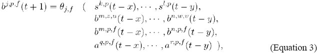

 the input variable ek represented in Ep;