ABSTRACT. Statistical tests that detect and measure deviation from the Hardy-Weinberg equilibrium (HWE) have been devised but are limited when testing for deviation at multiallelic DNA loci is attempted. Here we present the full Bayesian significance test (FBST) for the HWE. This test depends neither on asymptotic results nor on the number of possible alleles for the particular locus being evaluated. The FBST is based on the computation of an evidence index in favor of the HWE hypothesis. A great deal of forensic inference based on DNA evidence assumes that the HWE is valid for the genetic loci being used. We applied the FBST to genotypes obtained at several multiallelic short tandem repeat loci during routine parentage testing; the locus Penta E exemplifies those clearly in HWE while others such as D10S1214 and D19S253 do not appear to show this.

Key words: Dirichlet distribution, full Bayesian significance test, Hierarchical sequential testing, Hardy-Weinberg equilibrium

INTRODUCTION

The present report is the natural sequel to that of Montoya-Delgado et al. (2001) who introduced an exact significance test for the Hardy Weinberg equilibrium (HWE), reconciling Bayesian and frequentist ideas. For a complete description of the HWE, see Weir (1996). The Bayes factor was used to define an order in the sample space, and the sampling probability function utilized to compute the P value was the weighted likelihood average (for every possible sample point) over P_H, the null hypothesis subset of the parameter space. This test was originally presented by Pereira and Wechsler (1993), and its use with line integrals was discussed by Irony and Pereira (1995). The main limitations of this test are its strong dependence on the stopping rule (a violation of the likelihood principle) and on the parameterization being used. The present study presents a genuine Bayesian significance test, the full Bayesian significance test (FBST), introduced by Pereira and Stern (1999). In fact, we describe the invariant version of the FBST presented by Madruga et al. (2003).

A complete bibliographic discussion on the many HWE tests has been presented by Montoya-Delgado et al. (2001). Here, we restrict ourselves to describing and to applying the FBST to genotypes obtained at three multiallelic short tandem repeat (STR) loci: the locus Penta E exemplifies those clearly in HWE, while others such as D10S1214 and D19S253 do not.

The use of the FBST was applied here to define the loci that will be used for parentage testing. Note that the sample size of this kind of database is not fixed beforehand. Hence, the sample spaces were not completely defined, avoiding the use of frequentist methods.

Our study is based solely on the likelihood effectively obtained for any existing database size. The prior we use is the non-informative uniform density in the natural parameter space, making the likelihood the main element of our concerns. We understand the natural parameter space to be the one where the prior is assessed. Here, for example, the vector of populational genotype proportions is the natural parameter of interest. That is, suppose that there are m (a positive integer) possible alleles. There will be in this case k=m(m+1)/2 possible genotypes. The natural parameter space in this case is the simplex:

In the second section, we describe the likelihood, the hypothesis of interest, and the probability distributions involved. Subsequent sections describe the FBST and illustrate it with the case of biallelic loci, and review the hierarchical testing for multiple alleles as presented by Montoya-Delgado et al. (2001). The last section presents the results for three multiallelic STR loci: Penta E (Bacher et al., 2000), D10S1214 (Genbank accession number G08824) and D19S253 (Genbank accession number L13122).

DATA COLLECTION

Genomic DNA was obtained from unrelated, predominantly Caucasian individuals undergoing paternity testing nationwide by Genomic Engenharia Molecular Ltda. Alleles were amplified using fluorescently labeled primers, separated on DNA sequencing gels by electrophoresis, and visualized using an automatic DNA sequencer. Allele sizing was performed by running adjacent allelic ladders.

MODEL AND HYPOTHESIS

Let us consider the case of a locus with m possible alleles: a₁, a₂,…, a_m. The populational relative frequency of genotype (a_i,a_j), i £ j =1, 2,…, m is denoted by 0 £ p_ij £ 1. Since each individual that enters the process of evaluation is classified in one of the k=m(m+1)/2 possible genotypes, and by denoting the absolute frequency of individuals with genotype (a_i,a_j) as x_ij (a positive integer), the actual likelihood is given by

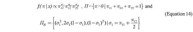
where p = (p_ij) and x =(x_ij), i £ j =1,…, m are the parameter and the sample frequency vectors, respectively.

For someone who will use only experimental information to assess his/her prior, the Dirichlet is the appropriate class of distribution to obtain the prior. That is, if a priori p has a Dirichlet distribution of order k with parameter d=(d_ij), i £ j =1,…, m and d_ij > 0, a posteriori p also has a Dirichlet distribution of order k but with parameter D = d+x. Note that for the uniform case where d=1 (the unity vector), the posterior density is the normalized likelihood that is the Dirichlet of order k with parameter x+1.

For the three databases that will be analyzed, the sample size is very large and the uniform prior is used. In this case, a deep study of the posterior corresponds to a deep study of the likelihood. This could go in the direction of the ideas of Fisher (1973).

To say that a locus is in HWE is to say that for any genotype (a_i,a_j) its populational frequency satisfies

where 2s_i =p_1i+…+p_(i-1)i+2p_ii+p_i(i+1)+…+ p_im.

Note that the dimension of the parameter space is k-1, and that the set of parameter points that satisfy the hypothesis, P_H, belongs to a subspace of dimension equal to m-1. Since m-1 < k-1, this is a sharp hypothesis. The main objective of the FBST is to test this sharp hypothesis.

Before ending this section, let us list some interesting quantities derived from the adoption of Dirichlet priors.

i) The posterior mean of p_ij is e_ij = E{p_ij½x} = D_ij /1´D, where 1´D is the sum of the components of D. (Equation 4)

ii) The posterior covariance matrix of p is Cov(p½x)= (diag(e)-ee´)/(1´D+1), where e is the vector (e_ij). (Equation 5)

iii) The posterior mode is the vector M=(D -1)[(1´D) - k)]^-1. (Equation 6)

iv) The maximum of the posterior inside the HWE hypothesis is the vector P=(p_ij), where, for D_i= D_1i+… +D_(i-1)i+2D_ii+D_i(i+1)+…+D_im and 2p_i=(1´D)^-1D_i, we have p_ij=2p_ip_j for i < j and p_ii = (p_i)². (Equation 7)

FBST for the HWE

Let p (Î P Í Â^k ) be the parameter vector of interest and L(p½x) the likelihood function associated with the observed data x, a standard statistical model. Under the Bayesian paradigm, the posterior density, ƒ_x(p), is proportional to the product of the likelihood and the prior density, ƒ(p). That is,

The (null) hypothesis H states that the parameter p lies in the null set, P_H Ì P. Usually the null set is defined by inequalities and equality constraints like the ones that define the HWE presented in the previous section. As in the case of the HWE, we are particularly interested in sharp (precise) null hypotheses, i.e., P_H belongs to a subspace with smaller dimension than the subspace where P was defined. Note that for the HWE, dim(P_H ) = m-1< k-1=dim(P). (Equation 9)

The FBST value of evidence in favor of H, Ev(H½x), is defined as follows:

· Let r(p) be an arbitrary density function, called here reference density. Usually, when working in the natural parameter space, we either take r(p) µ 1, i.e., the uniform density, or the non-informative prior if one is available. The reference density should not to be confused with the prior density, for the latter can be an informative density.

· Consider S_x(p) = ƒ_x(p)/r(p) as the posterior surprise function relative to the reference density r(p) and find the maximum inside the null set, a vector P Î P_H such that " p Î P_H gives

· Define the highest relative surprise set (HRSS) as

· The evidence against H is given by:

· Finally, the evidence in favor of H is given by

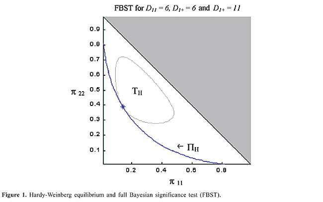
The surprise function has been discussed by Good (1983) and used by Evans (1997). In both papers, the reference density is exactly equal to the prior density. In that case, the surprise is related solely to the likelihood, avoiding the influence of the prior information. In our definition, when using the uniform reference density and the prior both in the natural parameter space, this prior information is highly considered even for complicated alternative parameterizations. The role of the surprise function here is to make Ev(H½x) explicitly invariant under suitable transformations on the coordinate system of the parameter space. The proof of this fact is not difficult and can be found in the study of Madruga et al. (2003).

The HRSS, T_H, contains the points of the parameter space, P, with higher surprise, relative to the reference density, r, than any point in the null set P_H. When r(p)=1, T_H is the posterior highest density probability set tangential to the null set P_H.

The evidence against H, Ev(H½x), gives an evaluation of the inconsistency between the posterior and the null hypothesis, and its complement is what we call the evidence in favor of H. A large value of Ev(H½x) indicates that the set of parameter points with higher density than the null hypothesis has high probability. Hence, large (small) values of Ev(H½x) disfavor (favor) H.

The HWE is a good illustration of the statistical appropriateness of the FBST. It is a non-linear hypothesis in a space of high dimension. Figure 1 illustrates the biallelic case showing the null and the tangential sets. This case was first discussed by Pereira and Stern (1999). Madruga et al. (2003) later showed, for a fixed sample size (the trinomial case), that the FBST should be the most powerful test for the HWE. Also, Madruga et al. (2001) showed that the FBST is a Bayesian test and thus a minimum risk (optimal) procedure.

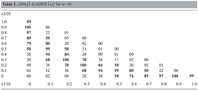
Table 1 presents the figures for the biallelic case with sample size n = 10. We present it here merely to give a flavor of the evidence calculus. For this example, we consider uniform prior and reference densities, r(p) = ƒ(p) =1. Recall that

Several other applications of the FBST, details of its numerical implementation, suggestive remarks regarding its epistemological implications, and an extensive list of references can be found in the authors’ previous publications.

Hierarchical sequential testing for HWE

In the previous section, we presented a simple method for computing an evidence index in favor of a sharp null hypothesis. Note that there is no restriction about dimensionality or sample size. However, the computational work will increase exponentially with an increasing number of alleles at a locus. For instance, for two alleles we have 3 genotypes, for 3 alleles we have 6 genotypes, for 4 alleles we have 10 genotypes and for m alleles we have k = m(m+1)/2 genotypes. To simplify this study we will use some of the Dirichlet properties. Let us review them here.

Let P be the simplex {(p₁,…,p_k) ½ p_I >0 & p₁+…+p_k=1} and define a random vector p assuming values on P with density function

where d = (d₁,…,d_k) is a vector of positive real numbers and G(a) is the gamma function evaluated at point a >0. The random vector p is said to have a Dirichlet distribution of order k with parameter d Î Â^k We denote this statement by p ~ Dir_k(d), and by x ~ y we mean that x and y have the same distribution.

Property 1

Let y = (y₁,…,y_k) a random vector of k independent random variables and s = y₁+…+y_k. For i = 1,…,k, let y_i be gamma distributed with shape parameter d_i > 0 and scale parameter b > 0. Then, by letting (1/s)y = p and d=(d₁,…d_k), for any choice of b, we have (1/s)y = p ~ Dir_k(d). (Equation 16)

We will state the next property in the context of the HWE problem. However, it is a very general property and uses Property 1 repeatedly in its proof. Here again, we define the vectors p and D of order k as before; p = (p_ij) and D=(D_ij), i < j =1,…,m with k=m(m+1)/2. Consider now the following appropriate notation:s₁+ =p₁₂+…+p_1m, p₁₊=(p₁₂,…,p_1m)(1/ s₁₊), s_1~ = 1- p₁₁ - s₁₊ , and p_1~=(1/s_1~)p⁽¹⁾, where p⁽¹⁾ is the vector (p_ij)_2£i£j£m. Also let D₁₊ = (D₁₂,…D_1m), D_1~ = (D_ij)_2£i£j£m. The sum of the components of these two vectors are denoted by 1´D₁₊ and 1´D_1~.

Property 2

The following two statements are equivalent

i) p ~ Dir_k(D)

ii) The vectors (p₁₂ ; s₁₊ ; s_1~), p₁₊ and p_1~ are mutually independent and are distributed as: (p₁₂ ; s₁₊ ; s_1~) ~ Dir₃(D₁₁; 1´D₁₊ ; 1´D_1~), p₁₊ ~ Dir_(m-1)(D₁₊), and p_1~ ~ Dir_(k-m)(D₁₊).

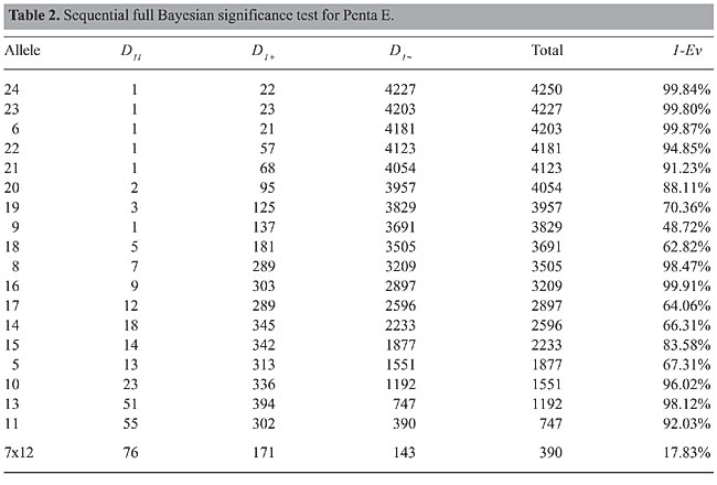
To prove these two important properties, one can use the techniques described by Basu and Pereira (1982). The first property is an application of Basu’s theorems (Basu, 1982). The second needs only simple algebraic uses of the first property.

The partition introduced by Property 2 is the basis of the method we will present in the sequel. We follow the same practical ideas of Montoya-Delgado et al. (2001). Note that the HWE only influences the vectors (p₁₂ ; s₁₊ ; s_1~) and p_1~. The vector p₁₊ is not affected by the occurrence of HWE. Our procedure follows the steps below:

Step 1

Without loss of generality, call a₁ the least frequent allele in the sample S in evaluation.

Step 2

Partition the sample S into three mutually exclusive sets:

S₁₁, all individuals with genotype (a₁,a₁);

S₁₊, all individuals with genotype (a₁,a_i), i >1, and

S_1~, all individuals with genotype (a_i,a_j), 2£ i £ j.

Step 3

Apply the FBST to (p₁₂ ; s₁₊ ; s_1~) ~ Dir₃(D₁₁; 1´D₁₊ ; 1´D_1~). Note that number of elements of each of these sets together with the prior parameters will produce the values of D₁₁, 1´D₁₊ , and 1´D_1~ . If the value of Ev is large enough to decide against H, declare the population to be in disequilibrium in relation to allele a₁. In this case, a₁ is one of the alleles responsible for this disequilibrium. If 1-Ev is large, declare that the population is in equilibrium.

Step 4

If S_1~ is composed of elements with only one allele involved, stop testing. If more than one allele is involved in the elements of S_1~ , rename S_1~ as S and go to Step 1.

With the procedure described, we will apply the FBST m-1 times and will have an idea of which alleles are producing the disequilibrium. In the next section, we apply the method to three sets of data: STR loci Penta E, D10S1214 and D19S253.

EXAMPLES

This section is devoted to the use of the method introduced in the previous sections. We chose three STR loci to discuss the use of FBST in sequence as described before. The first locus, Penta E, has m=20 possible alleles and k=210 genotypes and it is in HWE, since for all alleles the evidence in favor of HWE is high. The second locus D10S1214 has m=47 and k=1128. In this case, a large number of alleles are in disequilibrium, since the evidence in favor of HWE is very small. The third example, D19S253, has m=14 and k= 105. Also in this case, although having a small number of alleles, the evidence in favor of HWE is very small. Hence, we believe that Penta E is in equilibrium while the other two loci are not. Here we consider the prior and reference densities uniform.

Example 1: locus Penta E

Table 2 presents the results of the application of FBST for all alleles of Penta E. As we can see, most of the alleles show substantial evidence in favor of H, 1-Ev. Only when we test alleles 7 and 12 do we obtain a number between 15 and 20%. This is not enough to reject HWE. The conclusion is that this locus is in HWE.

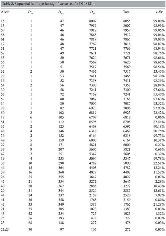
Example 2: locus D10S1214

Table 3 presents the results of the application of FBST for all alleles of D10S1214. In this locus we have 15 of 47 alleles in disequilibrium. The conclusion is that this locus is not in HWE.

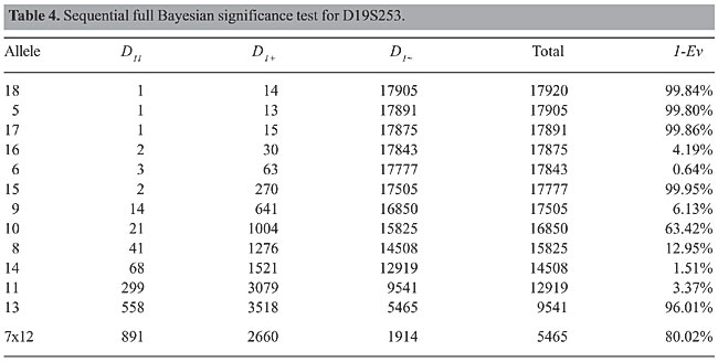
Example 3: locus D19S253

Table 4 presents the results of the application of FBST for all alleles of D19S253. In this locus we have 5 of 14 alleles in disequilibrium. The conclusion is that this locus is not in HWE.

If the reader wishes to compare the results presented here with other testing techniques, the original data can be found at http://www.ime.usp.br/~cpereira. A program for the biallelic HWE is also available at this site.

FINAL REMARKS

This paper introduces the FBST to the biostatistics environment. The motivation for the use of this test was the fact that the sampling space is not known in most cases since the stopping rule usually is not known. However, the FBST may be applied in any of the standard statistical situations as seen in our list of published papers (Pereira and Stern, 1999, 2001a,b,c; Irony et al., 2001; Stern and Zacks, 2002; Lauretto et al., 2003; Madruga et al., 2001, 2003; Rodrigues, 2006).

Before we list properties of the FBST, we recall that here we use the power of Dirichlet properties. These properties and their use may be found in Wilks (1968), Basu (1982), Basu and Pereira (1982), and Irony et al. (2000). For Bayesian statistics background we recommend Zellner (1971) and Press (1989).

In the applications discussed in this paper and in other previous papers, it is desirable or necessary to use a test with the following characteristics:

· Be formulated directly in the natural parameter space.

· Take into account the full geometry of the null hypothesis as manifold (surface) embedded in the whole space where the parameter space is defined.

· Have an intrinsically geometric definition, independent of any non-geometric aspect, such as the particular parameterization of the manifold representing the null hypothesis being evaluated.

· Be consistent with the Benefit of Doubt juridical principle (or Safe Harbor Liability rule). That is, one should consider in the “most favorable way” the claim stated by the hypothesis. Recall that T_H is the set of all parameter points with higher posterior density than the point in P_H with maximum density. Our judgment of H is based on the value of the posterior probability of T_H .

· Consider only the observed sample, respecting the likelihood principle, and allowing no ad hocery, such as a positive prior probability on the precise hypothesis. Recall that dim(P_H) < dim(P_H).

· Consider the alternative hypothesis in equal standing with the null hypothesis, in the sense that increasing sample size should make the test converge to the right (accept/reject) decision. Recall that for open-minded priors (positive densities for all possible values of p), the posterior density converges to Pr(p = p) =1, where p is the true value of p. In fact, P_H converges to a single point, the true value of the parameter in the case of an open-minded prior.

· Give an intuitive and simple measure of significance for the null hypothesis, ideally a probability in the parameter space, 1-Ev in our case.

· Allow the construction of an optimal decision rule. The decision of rejecting H whenever 1-Ev £ a for a fixed a, is in perfect harmony with the Bayesian decision theory of Rubin (1987), as shown by Madruga et al. (2001). This decision rule, when a stopping rule is well defined, is the most powerful test in the frequentist paradigm (Madruga et al., 2003).

· Be invariant under alternative parameterizations. The original definition of the FBST introduced by Pereira and Stern (1999) did not employ the reference density r. With the introduction of r and the consideration of HRSS, the invariance problem was solved.

The FBST has all these theoretical characteristics and has a straightforward computational implementation. It takes place entirely in the parameter space where the scientist assesses his/her prior density. We call it natural parameter space while acknowledging that the parameterization choice for the statistical model semantics is somewhat arbitrary.

We recall that the aim of most alternative parameterizations is to eliminate nuisance parameters, which can be achieved by conditioning, marginalization, or integration. The latter is most often used when building tests with Bayes factors, a traditional Bayesian method introduced by Jeffreys (1961), where a positive probability mass is assumed for P_H, producing Lindley’s paradox (Lindley, 1957). Usually, the hypothesis is projected onto a single point producing great simplification (Lindley, 1988). Basu (1977) and Pereira and Lindley (1987) discuss problems associated with these traditional methods. Usually, the natural parameter space allows no space for these ad hoc methods. The FBST is in sharp contrast with these traditional schemes of dimensional reduction. In fact the FBST preserves the natural parameter space in its full dimensionality. This property is key for an intrinsic regularization mechanism in the context of model selection (Pereira and Stern, 2001a,b).

Of course, there is a price to be paid for working with the full dimensionality of the parameter space: a considerable computational workload. Computational difficulties can be overcome with the use of efficient continuous optimization and numerical integration algorithms. Large problems can also benefit from program vectorization and parallelization techniques. We did not use these techniques here but instead employed a simplification of the problem using the factorization of the posterior density. We believe that, by considering the Dirichlet model, its factors following the HWE will imply the equilibrium in the whole space. Certainly, if one of the factors is in disequilibrium, the whole space then will also be in disequilibrium.

REFERENCES

Bacher JW, Helms C, Donnis-Keller H, Hennes L, et al. (2000). Chromosome localization of CODIS loci and new pentanucleotide repeat loci. Prog. Forensic Genet. 8: 33-36.

Basu D (1977). On the elimination of nuisance parameters. J. Am. Stat. Assoc. 72: 355-366.

Basu D (1982). Basu theorems. In: Encyclopedia of statistical sciences (Johnson NL and Kotz S, eds.). John Wiley and Sons Inc., New York, NY, USA, pp. 193-196.

Basu D and Pereira CAB (1982). On the Bayesian analysis of categorical data, the problem of nonresponse. J. Stat. Plann. Inference 6: 345-362.

Evans M (1997). Bayesian inference procedures derived via the concept of relative surprise. Commun. Stat. 26: 1125-1143.

Fisher RA (1973). Statistical methods and scientific inference. 3rd edn. Hafner Publishing Company, New York, NY, USA.

Good IJ (1983). Good thinking: the foundations of probability and its applications. University of Minnesota Press, Minneapolis, MN, USA.

Irony TZ and Pereira CAB (1995). Bayesian hypothesis test: using surface integrals to distribute prior information among hypotheses. Resenhas 2: 27-46.

Irony TZ, Pereira CAB and Tiwari RC (2000). Analysis of opinion swing: comparison of two correlated proportions. Am. Statistician 54: 57-62.

Irony TZ, Lauretto M, Pereira CAB and Stern JM (2001). A weibull wearout test: full Bayesian approach. In: System and Bayesian reliability: essays in honor of Richard Barlow on his 70th birthday (Hayakawa Y, Irony TZ and Xie M, eds.). World Scientific, Singapore, Malaysia, pp. 287-298.

Jeffreys H (1961). Theory of probability. 3rd edn. Clarendon Press, Oxford, England.

Lauretto M, Pereira CAB, Stern JM and Zacks S (2003). Comparing parameters of two bivariate normal distributions using the invariant FBST. Braz. J. Probab. Stat. 17: 147-168.

Lindley DV (1957). A statistical paradox. Biometrika 44: 187-192.

Lindley DV (1988). Statistical inference concerning Hardy-Weinberg equilibrium. Bayesian Stat. 3: 307-326.

Madruga MR, Steves LG and Wechsler S (2001). On the Bayesianity of Pereira-Stern tests. Test 10: 291-299.

Madruga MR, Pereira CAB and Stern JM (2003). Bayesian evidence test for precise hypotheses. J. Stat. Plann. Inference 117: 185-198.

Montoya-Delgado LE, Irony TZ, Pereira CAB and Whittle MR (2001). An unconditional exact test for the Hardy-Weinberg law: sample-space ordering using the Bayes factor. Genetics 158: 875-883.

Pereira CAB and Lindley DV (1987). Examples questioning the use of partial likelihood. Statistician 36: 15-20.

Pereira CAB and Wechsler S (1993). On the concept of P-value. Braz. J. Prob. Statist. 7: 159-177.

Pereira CAB and Stern JM (1999). Evidence and credibility: full Bayesian significance test for precise hypotheses. Entropy 1: 99-110.

Pereira CAB and Stern JM (2001a). FBST regularization and model selection. Annals of the 7th International Conference on Information Systems Analysis and Synthesis (ISAS 2001), Orlando, Florida, FL, USA, 7: 60-65.

Pereira CAB and Stern JM (2001b). Model selection: full Bayesian approach. Environmetrics 12: 559-568.

Pereira CAB and Stern JM (2001c). Full Bayesian significance tests for coefficients of variation. In: Bayesian methods with applications to science, policy, and official statistics. 6th World Meeting: Bayesian Techniques in Public Policy and Government (George EI, ed.). ISBA, Hersonissos, Crete, Greece, pp. 391-400.

Press SJ (1989). Bayesian statistics: principles, models, and applications. John Wiley and Sons Inc., New York, NY, USA.

Rodrigues J (2006). FBST for zero-inflated distributions. Commun. Stat. - TM 35: 1-9.

Rubin H (1987). A weak system of axioms for “rational” behavior and the nonseparability of utility and prior. Stat. Decisions 5: 47-58.

Stern JM and Zacks S (2002). Testing the independence of Poisson variates under the Holgate bivariate distribution: the power of a new evidence test. Stat. Prob. Lett. 60: 313-320.

Weir BS (1996). Genetic data analysis II. Sinauer Associates Inc., Sunderland, MA, USA.

Wilks SS (1968). Mathematical statistics. John Wiley and Sons Inc., New York, NY, USA.

Zellner A (1971). An introduction of Bayesian inference in econometrics. John Wiley and Sons Inc., New York, NY, USA.