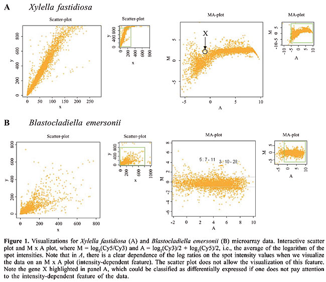
SpotWhatR: a user-friendly microarray data analysis system

INTRODUCTION

There are many different technologies that allow us to measure gene expression at the transcriptional and translational levels in a high-throughput framework. DNA microarrays have been widely used and have become very popular among scientists to measure gene expression or to perform genomic comparative studies. The principle of this technique is competitive hybridization between a control and a test sample, labeled with different fluorophores, Cy3 or Cy5, performed on a glass slide containing DNA fragments representing thousands of genes. In recent years, this technology has been improved in all steps: microarray construction, cDNA labeling, hybridization, fluorescence detection, as well as data acquisition and analysis (Bowtell, 1999; Holloway et al., 2002).

Microarray construction can be performed by robots (spotters) that deposit the DNA on a glass slide (Cheung et al., 1999) or by photolithography (Lipshutz et al., 1999). Initially, the DNA fragments immobilized on the slides were double-stranded PCR products; nowadays, most of them contain immobilized oligonucleotides, and there are also slides that present a 3-dimensional structure (Ramakrishnan et al., 2002). Labeling procedures have also improved to overcome differential incorporation rates of fluorophores (Holloway et al., 2002). There are various types of scanners available for fluorescence detection, some use lasers, and others use CCD cameras coupled to specific wavelength filters. Once the images have been acquired, there are numerous image analysis softwares that perform segmentation and spot fluorescent intensity quantification (Yang et al., 2001). In addition, there is also an increasing number of tools available for microarray data analysis, ranging from simple ones to more elaborate ones that involve neural networks (Narayanan et al., 2002) and Bayesian analysis (Yang et al., 2004). The inclusion of all these steps in microarray experiments increases the potential and reliability of this technique.

We present SpotWhatR, a user-friendly, freely available microarray data visualization and analysis system that dispenses with the need for programming skills. It is implemented using the freely available R statistical language (http://www.r-project.org), and it can be easily used in Windows operational systems, using interactive menus. SpotWhatR offers graphical options to visualize the data, normalization procedures, methods to find differentially expressed genes, and clustering algorithms.

We implemented in SpotWhatR tools that were successfully used and tested on microarray datasets of the phytopathogen Xylella fastidiosa (Koide et al., 2004; Pashalidis et al., 2005) and the primitive fungus Blastocladiella emersonii (Ribichich et al., 2005). Many of the data analysis scripts have also been used in microarray data from sugar cane (Papini-Terzi et al., 2005) and Trypanosoma cruzi (Baptista et al., 2004), as we have rewritten the R scripts to fulfill the need for a user-friendly interface. The aim of developing SpotWhatR was to facilitate the data analysis procedure for those who are not familiar with computational programming. It allows the researcher to test and use various analysis procedures without the need for extensive programming. Moreover, since it is an open-source software, new tools can be easily added to SpotWhatR, giving researchers the flexibility to implement or complete the software, according to their own needs.

MATERIAL AND METHODS

R scripts

The scripts were written in R statistical language (http://www.r-project.org) using the cluster library. In order to build the user-friendly interface, we used the tcltk library for the Linux version and the functions winDialog and winMenuAdd for the Windows version.

Microarray construction, labeling, hybridization, and detection

The microarrays used as examples were derived from the Blastocladiella emersonii and Xylella fastidiosa Microarray Projects. They were constructed by immobilizing PCR products on type 7 glass slides (GE Healthcare) spotted at least in duplicate. Total RNA was isolated using TriZol (Invitrogen) and was reverse transcribed and labeled using a CyScribe Post-labeling kit (GE Healthcare). The labeled targets were applied on the microarray slides, covered with a 24 x 60-mm cover slip (Corning), hybridized at 42°C for 16 h and washed in increasing stringency conditions. Microarray slides were scanned with a Generation III DNA Scanner (Molecular Dynamics). Fluorescence mean intensity and surrounding mean background from each spot were obtained with the software Array Vision, version 6.0 (Imaging Research, Inc.). Unreliable spots were manually flagged.

RESULTS

SpotWhatR facilities

In this section, we describe the tools available in SpotWhatR, showing examples and graphical outputs provided by the program.

Data visualization

The raw data that result from a common two-color microarray experiment are a set of two monochromatic images, one for each dye, usually a .TIF file. The fluorescence intensities are codified in a grey scale, from 2⁰ to 2¹⁶, although there are other proprietary codification schemes. The resolution and image quality depend on the scanner performance. This raw data have to be analyzed by software capable of delimiting the spot boundaries, and of quantifying the intensity of the spot and background. Since various programs can be used, this step of data extraction from the images is the first one for data analysis (Yang et al., 2001; Hirata et al., 2002; Saeed et al., 2003). Once the microarray image has been acquired and quantified by an image analysis program, it is important to choose a graphical output style to visualize the data. When using SpotWhatR, one may have already extracted the intensity data from images.

SpotWhatR offers the user three different kinds of data visualization: the traditional Cy3 x Cy5 scatter plot, the traditional M x A plot and the Q x P plot. The user has to upload the non-normalized or the normalized data and click on the graphic option desired.

Besides the classical scatter plot, which shows the fluorescent intensity of Cy3 versus Cy5 channels (Figure 1, left panels), there are other plots that allow us to perform a richer visualization of microarray data. These graphics usually show the log ratio on the y-axis versus an overall measure of spot fluorescence intensity on the x-axis (Figure 1, right panels). This kind of visualization allows us to see eventual non-linear dependence between ratios and fluorescent intensities, which may indicate that by using only the ratio values to classify a gene as differentially expressed may not be sufficient. For example, in the graph shown in Figure 1, gene X shows a 3-fold difference in ratio values; however, the spot intensity is very weak. This kind of result is unreliable, since hybridization intensity is weak, and it can lead to the classification of the gene as differentially expressed. Since the estimation of the microarray expression ratio does not depend on the strength of the hybridization signal, but on the biological meaningful signal, these plots are also useful to determine the kind of normalization procedure to be performed on the data.

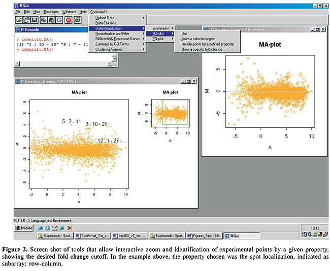
The graph used by Roberts et al. (2000) is one such example. The plot shows the logarithm of the expression ratio versus the logarithm of the mean intensity. Another useful and very common graphical display is the M x A plot, where M is defined as the log2(ratio) and A = log2(Cy3)/2 + log2(Cy5)/2 is the average of the logarithm of the spot intensities (Yang et al., 2002). As shown in the example below (Figure 1), it is possible to visualize the non-linear dependence of the spot intensities with the ratio values. SpotWhatR helps the user to see the systematic dependence of the ratio on intensity values. It can also help the user to determine the most suitable normalization procedure.

When we compare two populations in microarray experiments, there may be a situation in which a particular gene is not expressed in one condition, and thus the ratio values cannot be defined. One of the measured intensities is thus zero, and the usual ratios cannot be determined (e.g., Cy3/0 or Cy5/0 is not defined), yielding M = infinite value, which cannot be mathematically treated to compare data sets, and A = -infinity, which cannot be visualized in any graphical display.

To overcome this inconvenience, the data can be expressed in terms of two variables that represent the spot total intensity Q = Cy3 + Cy5 or its logarithm S = log2(Cy3/2 + Cy5/2) and the proportion of the hybridization of each target to a particular probe P = 1/(1 + 1/(normalized ratio)). In this kind of plot, we are already using the normalized ratio, since the raw ratio value would not be informative. The value of P is a non-linear transformation of the hybridization ratios, making these values limited to the 0 to 1 interval. To convert the variable P to the normalized ratio R, a simple algebraic manipulation is employed, where R = P/(1 - P). In the situation where one target is present in one of the channels and absent in the other, P = 1/(1 + 1/0) = 0 or P = 1/(1 + 0/1) = 1, avoiding infinite values. Without this adaptation, it would be impossible to visualize such absence/presence cases, which could be of major interest in practice.

In addition to the four different kinds of plots, there are also some other useful visualization tools, such as zooming, identifying points on the graph by a given property and showing a specific fold-change value. These tools help with data mining procedures, linking the graphical output with the rapid and practical identification of the points of interest, within a desired fold-change. In Figure 2, we show an example of the identification of some candidate outlier experimental points in an M x A plot.

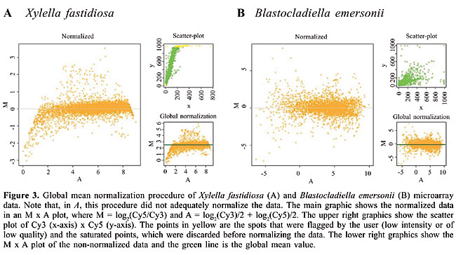
Normalization

The two-color microarray technology is based on the fluorescence of two different dyes, resulting in several types of imbalances, such as different incorporation efficiencies, wavelength detection and dye brightness. To overcome these problems, the data acquired from an image analysis program have to be normalized. There are various ways to normalize the data (Quackenbush, 2002; Yang et al., 2002), and it is up to the user to define the best method for each data set. SpotWhatR allows the user to choose between three different normalization procedures: global normalization, LOWESS and dye swap.

The hypothesis behind the first two procedures is that most genes should not change their expression value; the mean of the ratio values should be 1 (or log ratio = 0). However, depending on the biological context, this hypothesis may not hold. As shown by van de Peppel et al. (2003), under some experimental conditions there is a global shift of the ratio distribution, i.e., most genes may decrease or increase their expression by a constant value. This information would be lost if one assumes that there is no global change in gene expression. In these cases, it is better to use the dye-swap normalization procedure. SpotWhatR allows the user to filter the data before normalizing by determining a saturation cutoff and/or using a column labeled as FLAG, which is usually provided by the image analysis programs to mark low quality spots. We describe each available method:

· Global mean normalization

One of the easiest ways to perform normalization is to find a constant factor to correct all the spots in the data set, the so-called global normalization procedures. They correspond to a translation in the log-ratio values, in order to balance the two channel intensities. One example is to assume that the total intensity in the Cy3 channel should be equal to the total Cy5 intensity. Another example is to assume that the whole mean intensities should be equal. With this procedure, all the spots are corrected by a constant factor (Quackenbush, 2001). Figure 3 illustrates the global mean normalization for two different microarray datasets. The green line is the global mean value.

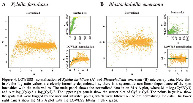
· LOWESS

When there is a systematic non-linear dependence between ratios and spot intensity values, it is appropriate to perform a normalization procedure that takes this systematic feature into account. This behavior can be visualized in the M x A (see the section on data visualization). Assuming that all the imbalances can be approximated by multiplicative factors that are contained in just one normalization constant that depends non-linearly on signal intensities, we can perform the LOWESS fitting on an M x A and obtain the normalization constant in an intensity-dependent framework (Yang et al., 2002). Figure 4 illustrates the LOWESS normalization procedure; the green line is the LOWESS fit on the non-normalized data; all the observed points are in orange, which are corrected to lead the fitted green points to M = 0. We observed that the LOWESS fitting normalized the Xylella fastidiosa dataset better than the global mean normalization (Figure 4A), since there was a clear intensity-dependent feature of the data, while both methods worked equivalently with the Blastocladiella emersonii dataset (Figure 4A and B).

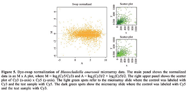
· Dye-swap

Since the normalization procedures are necessary due to differences in incorporation and dye brightness, the dye-swap procedure attempts to minimize this effect by labeling sample A with Cy3, B with Cy5 and also, in a separate experiment, A with Cy5 and B with Cy3. These hybridizations can be done as a control alone, or they can also be used to normalize the data. The dye swap normalization procedure consists of calculating the following ratio, using the results from dye swapped microarrays: R² = A²/B² = (Cy3/Cy5*k)/(k*Cy3/Cy5)_swap (Yang et al., 2002). One needs two experiments in order to obtain a single-expression ratio result. The advantage of this method is that there is no need to assume that most of the genes do not change their expression levels, which can be a more realistic approximation of the condition under test. The drawback is that one needs to perform all experiments in duplicate, preferably technical duplicates, to assure that the normalization constants k are in fact the same, and thus cancel each other out in the ratio equation above. It is prudent to perform at least some dye-swapping experiments, even if the normalization chosen is not the dye-swap procedure, to avoid artifacts in the differential expression detection procedure. Figure 5 illustrates the dye-swap normalization for Blastocladiella emersonii microarray data, performed by SpotWhatR.

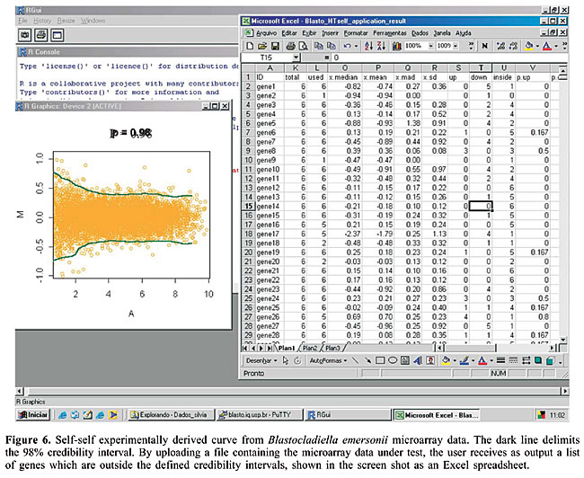
Finding differentially expressed genes

When analyzing a microarray dataset, a major question is how to classify a gene as differentially expressed. To answer this question, it is necessary to set a cutoff level for hybridization intensity ratios that permit one to decide whether a gene is differentially expressed or not. In mathematical terms, this step consists in testing the null hypothesis H₀: “the spot has no differential hybridization between the two probed samples”. SpotWhatR allows the user to find intensity-dependent cutoffs, by using self-self experiments or by determining outlier genes. This method was designed to provide a statistical analysis alternative to a low-replication dataset in which more elaborated known statistical methods, such as SAM (Tusher et al., 2001), are not recommended.

· HTself

Self-self experiments are performed by labeling the same biological material with either Cy3 or Cy5 dyes and hybridizing them simultaneously on the same microarray slide. This strategy has been used to derive intensity-dependent cutoffs to classify a gene as differentially expressed (Papini-Terzi et al., 2005; Pashalidis et al., 2005) or divergent in comparative genomic hybridization studies (Koide et al., 2004). The comparative analysis of constant fold change cutoffs and intensity-dependent ones has been extensively discussed, showing a superior performance of the intensity-dependent strategy. SpotWhatR provides the user with the HTself method (Vencio and Koide, 2005). Based on self-self experiments, the user can define intensity-dependent cutoffs with the desired credibility interval and obtain lists of differentially expressed genes. Figure 6 shows the self-self curve and its application to find differentially expressed genes using SpotWhatR.

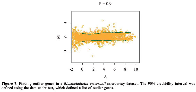
SpotWhatR could be considered as a stand-alone implementation of the HTself method. We refer the interested reader to the original work (Vencio and Koide, 2005) for a detailed explanation on this method.

· Outliers

Since microarray self-self experiments are not always performed, we also made available a method to find the outlier genes within an experiment. By defining the credibility interval using the data being examined, the user can find the genes that are more distant from the distribution than most, which can be useful to find differentially expressed genes. The rationale introduced by SpotWhatR is similar, where the genes that show the greatest fold change relative to the control are considered differentially expressed. For example, one could select the top 20% genes ranked by their fold change (the top 10% up-regulated plus the top 10% down-regulated), regardless of the magnitude of the fold change obtained. However, this simple rule could be very biased, due to the non-linear intensity dependence of the fold change with the fluorescence intensity, as discussed earlier. Therefore, the SpotWhatR outlier detection procedure works in an intensity-dependent framework, similar to the HTself method but using the data itself to define the cutoff curve, instead of the self-self curve. This procedure works as we selected the 20% greatest fold changes for each A interval in a sliding window (Figure 7). This percentage designation is a simplification, since the procedure is in fact more sophisticated: for example, as mentioned previously, it calculates the 80% credibility interval, which is different from simply sorting the fold changes and harvesting the top 20% genes.

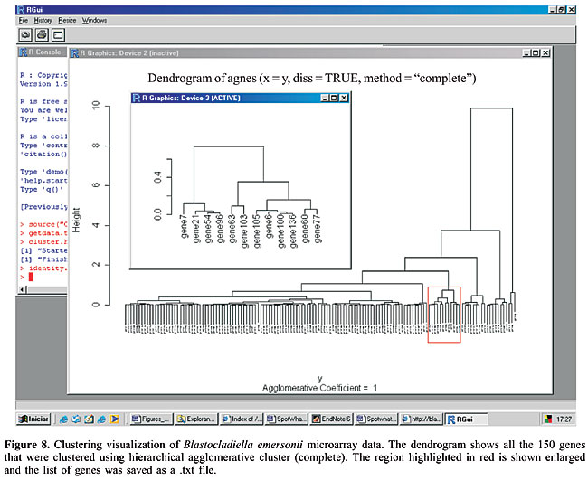
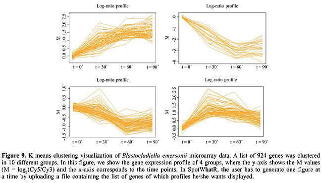
This procedure can be applied to non-normalized datasets, as long as the order of relations inside a small intensity window is maintained before and after the normalization process. In other words, in a given small intensity range, the genes that suffer the greatest fold changes are expected to be the same after normalization, since the outlier finding does not consider the numeric ratio obtained, but rather, the information of which gene appears first in an ordered list of genes. Multiplicative or additive operations do not change the list order.

Summary by Gene Ontology terms

A bioinformatics methodology that is becoming commonly used in microarray data analysis is the categorization of the result in ontology terms. The large outputs of high-throughput methods, such as lists of differentially expressed genes or cluster elements could be much more useful to biologists if summarized in ontology terms. The most common kind of term analyzed is the classification in gene categories, where the preferred scheme is the one proposed by the Gene Ontology (GO) Consortium (Ashburner et al., 2000).

In SpotWhatR, we have implemented a tool that summarizes a list of genes by GO terms or any other functional categorization familiar to the researcher. It allows the user to build a GO-to-gene table from a gene-to-GO table and to have GO statistics. It is very useful, mainly to those working with organisms that are not implemented in most of the on-line tools available (see a list of tools in http://www.geneontology.org/GO.tools.shtml). Since the user usually has a gene-to-GO table, SpotWhatR receives it as an input and builds a GO-to-gene table. SpotWhatR summarizes the data by giving the number of genes in each functional category; it also calculates the association measurement between “being differentially expressed” and “belonging to a given GO category”. This association measurement is calculated as described by Goodman and Kruskal (1954). Values near 1 indicate strong association. The output is a tab-delimited file (.txt), which can be easily manipulated in Excel spreadsheets.

Clustering

Clustering analysis is often performed to group genes that present similar expression patterns. This tool is very useful to explore the gene expression data, especially when it turns into a temporal series data set, allowing data visualization and the identification of patterns. There are plenty of clustering algorithms, and the choice of the most suitable one is still generally made in an empirical manner (Datta 2003). We believe that it is necessary to test different methods and choose one that helps the researcher to understand the biological processes under study. Moreover, the method should present a principle coherent with the structure of the data under analysis.

Clustering algorithms receive as input a similarity matrix, i.e., a matrix containing the distance between the vectors. In microarray data analysis, the similarity matrix contains the distance between gene expression profiles. We have implemented two different distance measures in SpotWhatR: the classical Euclidean distance and a distance that takes into account the replication measurements. The latter distance measure allows the user to incorporate the replication measurements to perform the clustering analysis, which will probably result in a more realistic data analysis (Yeung et al., 2003).

To perform the clustering analysis in SpotWhatR, the user must input a table with n lines (number of genes) and p columns, containing the gene names and the respective expression ratios. To use the distance measure that takes into account the replication, the user must also input another matrix containing the gene names and the respective error measurement, for example, standard deviation or median absolute deviation. Once the distance measurement is chosen, one of the following clustering methods can be performed: hierarchical agglomerative clustering, K-means, and DIANA. Our clustering algorithms are performed on the dataset with complete profiles to avoid errors that arise from data input, a classical and complex problem in clustering analysis (Troyanskaya et al., 2001). Since the clustering algorithms must have all the time points, many programs substitute them for constant values or means, which can influence the final result. The user can perform such an input process outside of SpotWhatR using his preferred tool and input this modified data into it for the clustering analysis. We prefer to work only with the reliable and complete time-series.

· Hierarchical agglomerative clustering

In this algorithm, the initial number of clusters is equal to the number of genes. Genes with similar expression profiles are successively grouped. Once a gene has been assigned to a particular group, there is no more mobility between groups and the distance is calculated relative to the group formed.

· DIANA

This is a divisive hierarchical clustering (DIvisive ANAlysis Clustering). In contrast to the agglomerative clustering, all the genes are initially assigned to a single group. At each step of the algorithm, the group is successively divided to form groups. The cluster with the highest dissimilarity is divided in each step, and the gene presenting the highest dissimilarity is identified to begin a new cluster. A gene can be moved from one cluster to another if the similarity with a new cluster is greater.

· K-means

This is an iterative clustering algorithm, where the number of clusters is one of the inputs of the algorithm. The user can define the number of groups. They are represented by centroids, the group center. The algorithm minimizes the sum of the distances of each object to the corresponding centroid. In each iteration, each gene is designated to the nearest centroid and new centroids are computed based on the gene distribution. These steps are repeated until there is no more mobility of the genes between the different clusters.

The output is a .txt file containing the gene name, description, the expression profile, and the number of the group.

SpotWhatR allows the user to visualize the cluster generated by the algorithms hierarchical and DIANA; one should click on the dendrogram display, select a cluster to be displayed enlarged and save the list of genes as a .txt file, as shown in Figure 8. This option is very useful to analyze the data and allow the user to have meaningful biological insights. For example, this list can be uploaded in the option Summarize by GO terms, allowing the researcher to see if there is an association between the genes in a cluster and their functional categorization. In addition, SpotWhatR allows gene expression profile visualization, as shown in Figure 9. Clustering algorithms require many calculations, thus, depending on the computer configuration and the number of genes, this option may take considerable time to be performed.

Script availability

To use SpotWhatR, one should first install R for Windows (http://lmq.esalq.usp.br/CRAN/) and download SpotWhatR at (http://blasto.iq.usp.br/~tkoide/SpotWhatR/). In the R environment, click “upload file”, and choose the spotwhat.R script file. Then, there will be a new item in the menu called SpotWhatR, which allows the utilization of our tool. The user can perform microarray data analysis by choosing the appropriate option in the interactive menu. Further detailed information and examples are available in the “SpotWhatR User Guide” in the supplemental web site.

DISCUSSION

Complex and high-throughput microarray datasets require data analysis tools capable of handling all the procedures necessary for an adequate analysis. Although the features of SpotWhatR are variants of existing methods, various are not easily available elsewhere. For example, the intensity-dependent outlier finding is a useful application that derived from the HTself method (Vencio and Koide, 2005). The clustering process considering the experimental replication is based on Yeung et al. (2003); however, their software does not allow an arbitrary and unbalanced number of experimental replicates for the different points in time series. Therefore, we implemented such an improvement.

SpotWhatR fulfills the need for a user-friendly interface for microarray data analysis. The scripts implemented in SpotWhatR were successfully used in various microarray datasets, such as Trypanosoma cruzi, sugar cane, Xylella fastidiosa, and Blastocladiella emersonii. However, we had to run scripts and alter some parameters manually, posing some difficulties to those not familiar with computational programming, impairing the test of different data analysis procedures that could be more suitable for the dataset. By implementing a user-friendly interface for Windows, we hope that other research groups can use this tool to analyze their microarray data. Moreover, since it is an open-source software, new tools can be easily added to SpotWhatR, giving researchers the flexibility to implement or complete the software, according to their needs.

REFERENCES

Ashburner M, Ball CA, Blake JA, Botstein D, et al. (2000). Gene ontology: tool for the unification of biology. The gene ontology consortium. Nat. Genet. 25: 25-29.

Baptista CS, Vencio RZ, Abdala S, Valadares MP, et al. (2004). DNA microarrays for comparative genomics and analysis of gene expression in Trypanosoma cruzi. Mol. Biochem. Parasitol. 138: 183-194.

Bowtell DD (1999). Options available - from start to finish - or obtaining expression data by microarray. Nat. Genet. 21 (Suppl 1): 25-32.

Cheung VG, Morley M, Aguilar F, Massimi A, et al. (1999). Making and reading microarrays. Nat. Genet. 21 (Suppl 1): 15-19.

Datta S and Datta S (2003). Comparisons and validation of statistical clustering techniques for microarray gene expression data. Bioinformatics 19: 459-466.

Goodman LA and Kruskal WH (1954). Measures of association for cross classifications. J. Am. Stat. Assoc. 49: 732-764.

Hirata Jr R, Barrera R, Hashimoto RF, Dantas DO, et al. (2002). Segmentation of microarray images by mathematical morphology. Real Time Imaging 8: 491-505.

Holloway AJ, van Laar RK, Tothill RW, Bowtell DD, et al. (2002). Options available - from start to finish - for obtaining data from DNA microarrays II. Nat. Genet. (Suppl 32): 481-489.

Koide T, Zaini PA, Moreira LM, Vencio RZ, et al. (2004). DNA microarray-based genome comparison of a pathogenic and a nonpathogenic strain of Xylella fastidiosa delineates genes important for bacterial virulence. J. Bacteriol. 186: 5442-5449.

Lipshutz RJ, Fodor SP, Gingeras TR, Lockhart DJ, et al. (1999). High density synthetic oligonucleotide arrays. Nat. Genet. 21 (Suppl 1): 20-24.

Narayanan A, Keedwell EC and Olsson B (2002). Artificial intelligence techniques for bioinformatics. Appl. Bioinformatics 1: 191-222.

Papini-Terzi FS, Rocha FR, Vencio RZ, Oliveira KC, et al. (2005). Transcription profiling of signal transduction-related genes in sugarcane tissues. DNA Res. 12: 27-38.

Pashalidis S, Moreira LM, Zaini PA, Campanharo JC, et al. (2005). Whole-genome expression profiling of Xylella fastidiosa in response to growth on glucose. OMICS 9: 77-90.

Quackenbush J (2001). Computational analysis of microarray data. Nat. Rev. Genet. 2: 418-427.

Quackenbush J (2002). Microarray data normalization and transformation. Nat. Genet. (Suppl 32): 496-501.

Ramakrishnan R, Dorris D, Lublinsky A, Nguyen A, et al. (2002). An assessment of Motorola CodeLink microarray performance for gene expression profiling applications. Nucleic Acids Res. 30: e30.

Ribichich KF, Salem-Izacc SM, Georg RC, Vencio RZ, et al. (2005). Gene discovery and expression profile analysis through sequencing of expressed sequence tags from different developmental stages of the chytridiomycete Blastocladiella emersonii. Eukaryot. Cell 4: 455-464.

Roberts CJ, Nelson B, Marton MJ, Stoughton R, et al. (2000). Signaling and circuitry of multiple MAPK pathways revealed by a matrix of global gene expression profiles. Science 287: 873-880.

Saeed AI, Sharov V, White J, Li J, et al. (2003). TM4: a free, open-source system for microarray data management and analysis. Biotechniques 34: 374-378.

Troyanskaya O, Cantor M, Sherlock G, Brown P, et al. (2001). Missing value estimation methods for DNA microarrays. Bioinformatics 17: 520-525.

Tusher VG, Tibshirani R and Chu G (2001). Significance analysis of microarrays applied to the ionizing radiation response. Proc. Natl. Acad. Sci. USA 98: 5116-5121.

van de Peppel J, Kemmeren P, van Bakel H, Radonjic M, et al. (2003). Monitoring global messenger RNA changes in externally controlled microarray experiments. EMBO Rep. 4: 387-393.

Vencio RZ and Koide T (2005). HTself: Self-self based statistical test for low replication microarray studies. DNA Res. 12: 211-214.

Yang YH, Buckley MJ and Speed TP (2001). Analysis of cDNA microarray images. Brief. Bioinform. 2: 341-349.

Yang YH, Dudoit S, Luu P, Lin DM, et al. (2002). Normalization for cDNA microarray data: a robust composite method addressing single and multiple slide systematic variation. Nucleic Acids Res. 30: e15.

Yang D, Zakharkin SO, Page GP, Brand JP, et al. (2004). Applications of Bayesian statistical methods in microarray data analysis. Am. J. Pharmacogenomics 4: 53-62.

Yeung KY, Medvedovic M and Bumgarner RE (2003). Clustering gene-expression data with repeated measurements. Genome Biol. 4: R34.